Want to become an expert in VBA? So this is the right place for you. This blog mainly focus on teaching how to apply Visual Basic for Microsoft Excel. So improve the functionality of your excel workbooks with the aid of this blog. Also ask any questions you have regarding MS Excel and applying VBA. We are happy to assist you.

Save a Workbook as a Single PDF Using VBA

From our last post we learnt how to convert an entire workbook to a single PDF manually. If you want to know how, then please check this post.

Convert an Entire Workbook to a Single PDF File

Today I’m going to teach you how to do the same thing using VBA. So you can use this subroutine inside your VBA applications where necessary. Now let’s start developing the code. First we need to declare a few variables.

We need to loop through all the sheets of the workbook. So we need to declare one variable as worksheet.

Dim WS As Worksheet

Then we need an array to assign sheet names.

Dim SheetNames() As Variant

PDF file name will be assigned to a string type variable.

Dim PDF_FileName As String

In addition to those variables, let’s declare two more variables of type integer. One is to hold the number of sheets. And other variable is to use as a counter inside for next loop.

Dim NumberOfSheets As Integer
Dim Counter As Integer

Now we have declared all the required variables. After variable declaration we can calculate the number of sheets inside the workbook as our first step.

NumberOfSheets = ThisWorkbook.Worksheets.Count

Now we know the upper bound of our SheetNames array. So we can size that dynamic array using redim statement.

ReDim SheetNames(1 To NumberOfSheets)

As our next step we can loop through all the sheets of the workbook and assign name of each worksheet to the SheetNames array. We can do it as follows.

Counter = 1

For Each WS In Worksheets
     SheetNames(Counter) = WS.Name
     Counter = Counter + 1
Next WS

Now let’s assign a name to our PDF file. You can give any valid name to the PDF file.


PDF_FileName = "PDf file name here"

Next we use SheetNames array to select all the sheets.

Sheets(SheetNames).Select

Then we can convert all the sheets to one single PDF file as follows.

ActiveSheet.ExportAsFixedFormat Type:=xlTypePDF, Filename:= _
"D:\Work\Create PDF\" & PDF_FileName & ".pdf", Quality:=xlQualityStandard, _
IncludeDocProperties:=True, IgnorePrintAreas:=False, OpenAfterPublish:= _
False

You should replace "D:\Work\Create PDF\" with path of your folder where you need to save the PDF file. Or else you can assign the folder path to a variable and then use that inside the code like this.

Dim FolderPath as string

FolderPath = "D:\Work\Create PDF"

ActiveSheet.ExportAsFixedFormat Type:=xlTypePDF, Filename:= _
FolderPath & "\" & PDF_FileName & ".pdf", Quality:=xlQualityStandard, _
IncludeDocProperties:=True, IgnorePrintAreas:=False, OpenAfterPublish:= _
False

Here is the complete subroutine.

Sub ConvertWorkbookToSinglePDF()

Dim WS As Worksheet

Dim SheetNames() As Variant

Dim PDF_FileName As String

Dim NumberOfSheets As Integer
Dim Counter As Integer

NumberOfSheets = ThisWorkbook.Worksheets.Count

ReDim SheetNames(1 To NumberOfSheets)

Counter = 1

For Each WS In Worksheets
     SheetNames(Counter) = WS.Name
     Counter = Counter + 1
Next WS

PDF_FileName = "PDf file name here"

Sheets(SheetNames).Select

ActiveSheet.ExportAsFixedFormat Type:=xlTypePDF, Filename:= _
"D:\Work\New Post 2\" & PDF_FileName & ".pdf", Quality:=xlQualityStandard, _
IncludeDocProperties:=True, IgnorePrintAreas:=False, OpenAfterPublish:= _
False

End Sub

Convert an Entire Workbook to a Single PDF File

Did you know that you can convert an entire Excel workbook to a single PDF. In this post I will teach you how to do that. First open your excel workbook. And the click on the “File” menu.


Then click on the “Save As” and browse for the folder.

Save As dialog box will open like this.

Give a suitable name for the PDF file from the file name field. And select PDF from the save as type field.

When you select the PDF, few more options will be available at the bottom of the Save As dialog box. Click on the options button.

When you click on the Options button excel will open Options window. Select entire workbook option from “Publish what” section (Default setting is Activesheet(s)). Then click OK. Options window will be closed.


Now click on the “Save” button of the “Save As” dialog box. Excel will convert all the tabs in the Excel workbook to a single PDF file.

VBA Int function

In a recent post we learnt a useful VBA function call Fix function. Today I’m going to explain about very similar function. Name of this new VBA function is Int. Like Fix function this also returns the integer part of the number. But there is a small difference between these two functions. These two functions behave slightly different when dealing with negative numbers. If there is a decimal place in a negative value then Fix function will return the first negative number greater than the value.

Ex -
Fix(-29.1) will return -29

If there is a decimal place in the negative value then Int function will return first negative number less than the value.

Ex -
Int(-29.1) will return -30

However both functions treat positive values in same manner.

Now let’s consider this below subroutine. We can get a clear idea about VBA Int function if we run it.

Sub IntFunctionExample()

Dim SampleValues(7) As Double

Dim i As Integer

SampleValues(0) = 0.32
SampleValues(1) = 5
SampleValues(2) = 7.1
SampleValues(3) = 7.8
SampleValues(4) = 0
SampleValues(5) = -15.1
SampleValues(6) = -15.9
SampleValues(7) = -30

For i = LBound(SampleValues) To UBound(SampleValues)
     Debug.Print Int(SampleValues(i))
Next i

End Sub

So if we run the above code it will show us below result in immediate window.

0
5
7
7
0
-16
-16
-30

Compare number arguments of the function and return values to understand how Int function works.

How to Check If a Value Has Decimal Places

In my last post I introduced you a useful VBA function call Fix. Today I’m going to show you how you can use that function to check whether a value has decimal places or not. In other words how to check whether a value is an integer/long or not.

I will explain this using an example. Let’s consider this array.

Dim SampleValues(4) As Double

SampleValues(0) = 5
SampleValues(1) = 5.95
SampleValues(2) = 20
SampleValues(3) = -13.7
SampleValues(4) = -2

So now let’s try to find out whether each value in this array has decimal place or not. We can do it like this.

Sub CheckForDecimalPlaces()

Dim SampleValues(4) As Double

Dim i As Long

SampleValues(0) = 5
SampleValues(1) = 5.95
SampleValues(2) = 20
SampleValues(3) = -13.7
SampleValues(4) = -2

For i = LBound(SampleValues) To UBound(SampleValues)
     If Fix(SampleValues(i)) = SampleValues(i) Then
         Debug.Print SampleValues(i) & " - No decimal places"
     Else
         Debug.Print SampleValues(i) & " - has decimal places"
     End If
Next i

End Sub

In above subroutine Fix function is used with an if statement. Let’s consider the following line.

If Fix(SampleValues(i)) = SampleValues(i) Then

So if we take the value 5 then Fix(5) equals to 5. Then 5=5. So above if statement becomes true. If we take the value 5.95 then Fix(5.95) equals to 5. But 5 is not equals to 5.95. So in that case above if statement becomes false.

That's how you can use Fix function to check whether a value has decimal places or not. So If we run above code we will get following result in the immediate window.

5 - No decimal places
5.95 - has decimal places
20 - No decimal places
-13.7 - has decimal places
-2 - No decimal places

VBA Fix Function

Today I'm going to explain you another very useful VBA function. It is Fix function. You can use this function to get the integer part of a numerical value. For an example, if you parse value 102.5 to the Fix function it will return 102

Here below is a sample subroutine from which you can get a clear idea about how this function works.

Sub FixFunctionExample()

Dim SampleValues(4) As Double

SampleValues(0) = 0.25
SampleValues(1) = 5.78
SampleValues(2) = 100.5
SampleValues(3) = -25.8
SampleValues(4) = -30.2

For i = LBound(SampleValues) To UBound(SampleValues)
Debug.Print Fix(SampleValues(i))
Next i

End Sub

If you run the above code, you will get following result in the intermediate window.

0
5
100
-25
-30

Change Font Color in VBA Editor in MS Excel

Did you know that you can change font colors in VBA editor. We can find various text types inside the VBA editor. These different text types have different font colors in default. Here is the complete list of text types you can find inside the VBA editor.


  • Normal Text
  • Selection Text
  • Syntax Error Text
  • Execution Point Text
  • Breakpoint Text
  • Comment Text
  • Keyword Text
  • Identifier Text
  • Bookmark Text
  • Call Return Text

In default, these various text types have different colors. However we have an option to choose colors for these text types according to our preference. So today I'm going to show you how to change font colors in VBA editor. First, launch your Excel application and create blank workbook. Then go to the VBA editor. You can click inside the spreadsheet and press Alt + F11 to use shortcut keys to open the VBA editor.

So this is a sample code I have written in a module.

As you can see, I'm using default text colors in VBA editor. Now let's see how to change the text colors inside the editor. Click on "Tools" menu and select "Options".

Then "Options dialog box" will open like this.

This dialog box has 4 tabs.

  • Editor
  • Editor Format
  • General
  • Docking

Editor tab is selected default. Now select the "Editor Format" tab.


As you can see different text types are listed under code colors. When you select a text type, font color of that text type is shown under the Foreground. In default, Normal text foreground color is set to Auto. If you select "Syntax Error Text" then Foreground will change to red like this.

Also sample text will be shown in the bottom right corner of the dialog box. So you can easily preview the formatting of the text when you do the changes.

Now let's change color of the "Normal Text". First select the "Normal Text" under code colors and then select color you want from the Foreground dropdown.

However as you can see there are limited number of colors we can choose for the font colors. So I selected different color for the "Normal text" and this is how my code looks like now.

In default, both "Normal Text" and "Identifier Text" have same font color. So if I change the "Identifier Text" to the same color as "Normal Text" then sample code will look like this.


Hide Worksheet Tabs in Excel

Sometimes we want to hide tab names in Excel workbooks. This is often needed when we developing applications similar to excel dashboards. Because in these applications we create custom buttons and hyperlinks to navigate between tabs. We usually disable the default tab navigation because it can interfere with the functionality of our application. Other reason is the appearance. Because we can create very professional looking navigation method instead of default tab names.

This is a sample navigation method I created using rectangle shapes and a vba macro.

sample dashboard with hidden tabs

This dashboard has several worksheets. But you can’t see the default tab names. So in this post I will explain you how to hide tabs names in an Excel file.

First click on the File menu.

File menu

Then click on Options.

Options

Excel Options dialog box will appear like this. Then select the Advanced category.

Select advance in excel options

Then scroll down to ”Display options for this workbook” section. Remove the tick from “Show sheet tabs” and click OK.

Remove tick from show sheet tabs

Then the default tab names will disappear. Before hide tabs you should create buttons or hyperlinks to navigate between tabs. Also note that this is a file level control. So if you want to remove default tab names for more than one file then you will need to do it for each file separately.

Sum Function (Worksheet)

In this post I’m going to show you how to use Sum function in excel worksheets.

Sum Function character

We use sum function to add values in Excel. Parameters for the sum function can be entered in few different ways. In this post I will show you these different methods one by one. Let’s consider this example sheet.

Sample data

So if we want to find total quantity using sum function, we can do it in few different ways. First method is we can directly enter the values inside sum function like this.

=SUM(9,10,4,6,3,8,1)

enter values directly in Sum function

Then we will get 41 as total.

Result

However if you use this method, total won’t change when you do changes to the quantities of the individual stones. So if you want to use sum function in such a way that total value changes when individual quantity of stones change, then you need to use cell references instead of direct values. Here is how you can do it.

=SUM(B2,B3,B4,B5,B6,B7,B8)

sum function with cell references

Now if you do any change to a individual quantity, it will be reflected in the total instantly. In above method we used individual cell references inside the Sum function. Next let's learn how to use ranges instead of individual cell references. You can simple replace cell references with the relevant range like this.

=SUM(B2:B8)

Sum function with range

In above example we used Sum function for contiguous range. So what if we want to use Sum function for non-contiguous range like this.

Non-contiguous range example data

I have highlighted the non-contiguous range in yellow. So now let’s learn how to use Sum function for this non-contiguous range. If we want to enter values directly then we can use Sum functions like we did earlier. So it will look like this.

=SUM(9,10,4,6,3,8,1,2,4,7,5)

And if we want to enter cell references then we can do it as follows.

=SUM(B2,B3,B4,B5,B6,B7,B8,E2,E3,E4,E5)

cell reference method in Sum function for non-contiguous range

And this is how you can enter range for Sum function for non-contiguous range.

=SUM(B2:B8,E2:E5)

Range input for Sum function for non-contiguous range

How to remove duplicates in excel

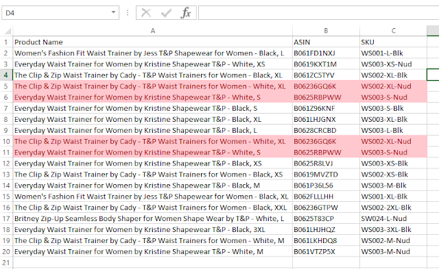
In this lesson I will explain you how to remove duplicates in excel. We often deal with excel or csv files which contain duplicate values. Sometimes duplicate values add meaning to the data. But sometimes these duplicates are troublesome. Specially when we analyze data. Now I will explain step by step, how to remove duplicates from your excel or csv files. Let’s consider this sample excel file. As you can see, I have highlighted the duplicates in this excel sheet.


Sample data with duplicate values

To remove duplicates, first click on one cell inside the data range. Then go to the “Data” tab and click on “Remove Duplicates”

Go to Data tab

“Remove Duplicates” dialog box will pop like this.

Remove duplicates dialog box

Select all the checkboxes and click OK. You will get result like this.

result data

Also we can do that using a vba macro as well. Below is the code to do that.

Sub RemoveDuplicates()

ActiveSheet.Range("$A$1:$C$20").RemoveDuplicates Columns:=Array(1, 2, 3), Header:=xlYes

End Sub

In above example, values will be removed only if columns A,B and C all have same data. Next let’s learn how to remove rows if a particular column has same data. Let’s consider this sample data set.

sample data

In this example sheet, I have highlighted the duplicate values we can find in column A. As you can see if we consider both column A and B then data are not same. In this example we are going to remove duplicates only based on column A. To do that first click on one cell within the data set. And then go to “Data” tab like in previous example and click on “Remove Duplicates”. Then remove duplicates dialog box will appear. In this dialog box only put tick to the “First Name” checkbox.

Remove duplicates dialog box

Then click OK and you will get this result.

Result data

Also you can use below macro to do it automatically as well.

Sub RemoveDuplicatesFromColA()

ActiveSheet.Range("$A$1:$B$17").RemoveDuplicates Columns:=1, Header:=xlYes

End Sub

How to Print Automatically (Excel VBA)

In this post I will explain how we can take printouts automatically using vba. So let’s consider this sample sheet.


This is a employee ID of a company. We use this ID as a template to generate IDs for each and every employee of the company. Now let’s look at how we can print this ID. We can do it easily like this.

Sub PrintID()

Dim WS As Worksheet

Set WS = Worksheets("Sheet2")

WS.Range("B2:J13").PrintOut

End Sub

Here "Sheet2" is the name of the worksheet. And Range("B2:J13") is the area we need to print. So you should modify the sheet name and range according to your worksheet name and range, you want to print. If you run above code it will print the ID automatically.

So we learned how to take printout of a range we want. But what if we need several copies of that range. We can take several copies automatically using following code. This below code will print 2 copies of that same range.

Sub PrintID_2Copies()

Dim WS As Worksheet

Set WS = Worksheets("Sheet2")

WS.Range("B2:J13").PrintOut Copies:=2

End Sub

Note that using this above code you can only print one ID. However if you need you can improve this macro to print IDs for all the employees in a database. Let’s assume you have a database with information of your employees. Then you can use For loop and cell addresses to create and print ID for each and every employee in that database.

Contact Form

Name

Email *

Message *