Hide Worksheet Tabs in Excel

Sometimes we want to hide tab names in Excel workbooks. This is often needed when we developing applications similar to excel dashboards. Because in these applications we create custom buttons and hyperlinks to navigate between tabs. We usually disable the default tab navigation because it can interfere with the functionality of our application. Other reason is the appearance. Because we can create very professional looking navigation method instead of default tab names.

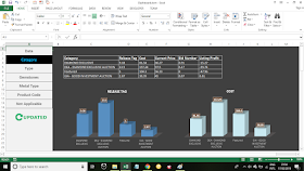
This is a sample navigation method I created using rectangle shapes and a vba macro.

This dashboard has several worksheets. But you can’t see the default tab names. So in this post I will explain you how to hide tabs names in an Excel file.

First click on the File menu.

Then click on Options.

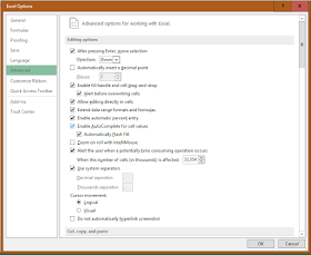
Excel Options dialog box will appear like this. Then select the Advanced category.

Then scroll down to ”Display options for this workbook” section. Remove the tick from “Show sheet tabs” and click OK.

Then the default tab names will disappear. Before hide tabs you should create buttons or hyperlinks to navigate between tabs. Also note that this is a file level control. So if you want to remove default tab names for more than one file then you will need to do it for each file separately.

Sum Function (Worksheet)

In this post I’m going to show you how to use Sum function in excel worksheets.

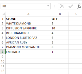
We use sum function to add values in Excel. Parameters for the sum function can be entered in few different ways. In this post I will show you these different methods one by one. Let’s consider this example sheet.

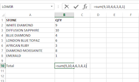
So if we want to find total quantity using sum function, we can do it in few different ways. First method is we can directly enter the values inside sum function like this.

=SUM(9,10,4,6,3,8,1)

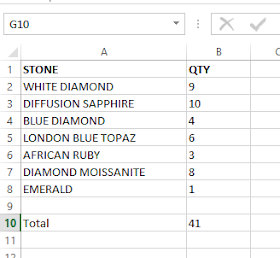
Then we will get 41 as total.

However if you use this method, total won’t change when you do changes to the quantities of the individual stones. So if you want to use sum function in such a way that total value changes when individual quantity of stones change, then you need to use cell references instead of direct values. Here is how you can do it.

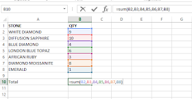
=SUM(B2,B3,B4,B5,B6,B7,B8)

Now if you do any change to a individual quantity, it will be reflected in the total instantly. In above method we used individual cell references inside the Sum function. Next let's learn how to use ranges instead of individual cell references. You can simple replace cell references with the relevant range like this.

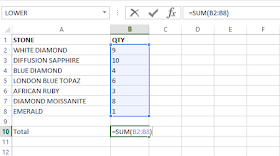
=SUM(B2:B8)

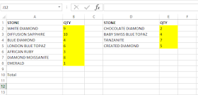
In above example we used Sum function for contiguous range. So what if we want to use Sum function for non-contiguous range like this.

I have highlighted the non-contiguous range in yellow. So now let’s learn how to use Sum function for this non-contiguous range. If we want to enter values directly then we can use Sum functions like we did earlier. So it will look like this.

=SUM(9,10,4,6,3,8,1,2,4,7,5)

And if we want to enter cell references then we can do it as follows.

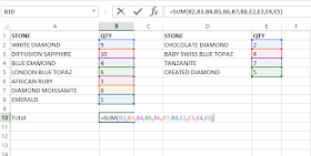
=SUM(B2,B3,B4,B5,B6,B7,B8,E2,E3,E4,E5)

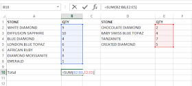
And this is how you can enter range for Sum function for non-contiguous range.

=SUM(B2:B8,E2:E5)