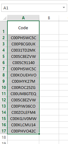
In this post you will learn about how to highlight duplicate values in Excel. Let’s consider this sample data.
This Excel sheet contains a list of codes in column A. Assume we want to know whether there are duplicated codes in the list and highlight them. Instead of manually examining, we can use conditional formatting available in the Excel application to highlight the duplicates. Follow the below steps.
First select the data set.
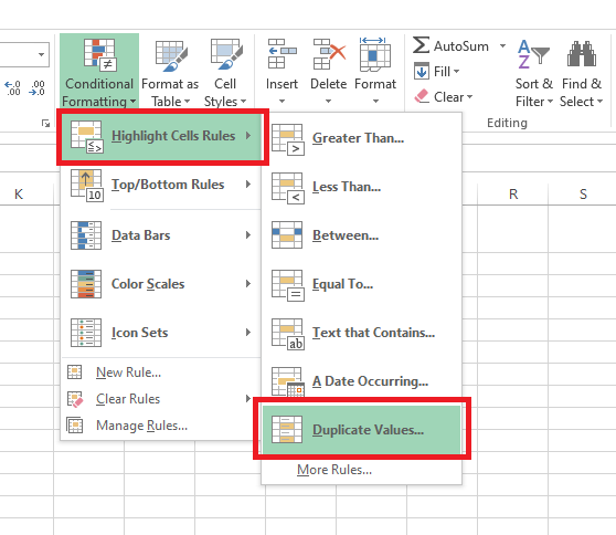
Then select the “Home” tab from the Excel ribbon.
Click on the “Conditional Formatting” in the style group.
Now take the cursor on top of the “Highlight Cells Rules” menu. Then a submenu will appear to the right. Click on the “Duplicate Values” from that submenu.
Then the Duplicate values window will open like this. Select “Duplicate” from the first dropdown. I will select “Light Red Fill with Dark Red Text” from the second dropdown. You can select any other format or custom format from the list.
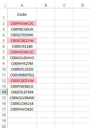
Then click the "OK" button. Duplicate codes will be highlighted like this.
In the above example we selected a range to apply the conditional formatting. However if you need you can add the conditional formatting to the entire column as well. To do that you need to change only one step. When selecting the data, select the entire column instead of the range. Below image shows how you should select the column.


